plot(model_lm, which = 1)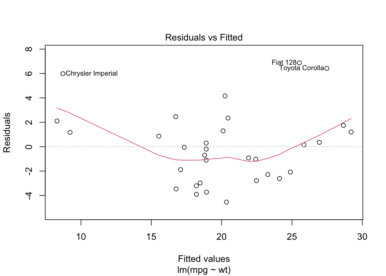
Course: PFRH 712 - Methods in Analysis of Large Population Surveys
Instructor: Dr. Saifuddin Ahmed
This lecture focuses on the principles and applications of design-based regression analysis using complex survey data in R. It introduces the correct use of lm(), glm(), and svyglm() functions with appropriate survey design using the survey package. It emphasizes best practices in model fitting, diagnostics, and interpretation, and highlights common pitfalls such as misuse of stepwise regression and pseudo R².
library(survey)
# Define the survey design
des <- svydesign(ids = ~psu, strata = ~strata, weights = ~weight, data = df)

# Linear regression
model_lm <- svyglm(gfr ~ cpr, design = des)
summary(model_lm)# Binary outcome model
model_logit <- svyglm(mcu ~ age + education, design = des, family = quasibinomial())
summary(model_logit)model_logbin <- svyglm(mcu ~ age + education, design = des, family = binomial(link = "log"))
summary(model_logbin)model_poisson <- svyglm(mcu ~ age + education, design = des, family = poisson(link = "log"))
summary(model_poisson)Residual vs Fitted Plot
plot(model_lm, which = 1)
Interpretation:
✅ Good fit if points scatter randomly around the horizontal line.
❌ Poor fit if there’s a curve or funnel shape (non-linearity or heteroscedasticity).
Q-Q Plot (Normality of Residuals)
plot(model_lm, which = 2)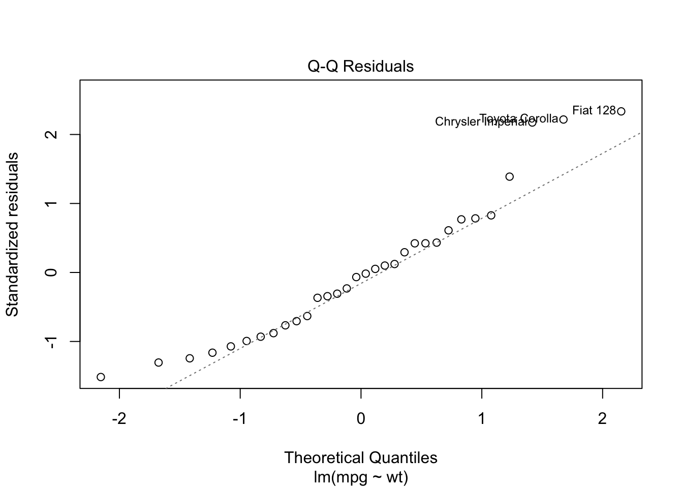
Interpretation:
✅ Good fit if points lie approximately on the diagonal line.
❌ Poor fit if points deviate at the ends (skewed distribution).
bptest(model_lm)
    studentized Breusch-Pagan test

data:  model_lm
BP = 0.040438, df = 1, p-value = 0.8406
Interpretation:
p > 0.05 → Homoscedasticity (good!)
p < 0.05 → Heteroscedasticity (bad — use robust SEs)
plot(model_lm, which = 4)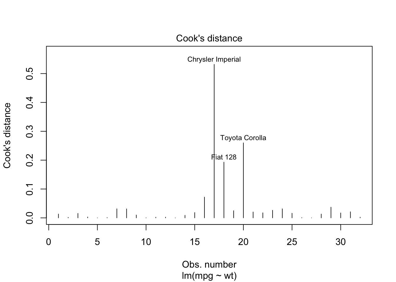
Interpretation:
model_logit <- glm(am ~ wt + hp, data = mtcars, family = binomial)
summary(model_logit)
Call:
glm(formula = am ~ wt + hp, family = binomial, data = mtcars)

Coefficients:
            Estimate Std. Error z value Pr(>|z|)
(Intercept) 18.86630    7.44356   2.535  0.01126 *
wt          -8.08348    3.06868  -2.634  0.00843 **
hp           0.03626    0.01773   2.044  0.04091 *
---
Signif. codes:  0 '***' 0.001 '**' 0.01 '*' 0.05 '.' 0.1 ' ' 1

(Dispersion parameter for binomial family taken to be 1)

    Null deviance: 43.230  on 31  degrees of freedom
Residual deviance: 10.059  on 29  degrees of freedom
AIC: 16.059

Number of Fisher Scoring iterations: 8
# Run Hosmer-Lemeshow test
hoslem.test(mtcars$am, fitted(model_logit))
    Hosmer and Lemeshow goodness of fit (GOF) test

data:  mtcars$am, fitted(model_logit)
X-squared = 4.9517, df = 8, p-value = 0.7627
Interpretation:
✅ p > 0.05 = model fits well
❌ p < 0.05 = poor fit
| Diagnostic | Good Fit | Poor Fit |
|---|---|---|
| Residual Plot | Random scatter | Curved / funnel shape |
| Q-Q Plot | Points near line | Points deviate |
| Breusch-Pagan Test | p > 0.05 | p < 0.05 |
| Cook’s Distance | All < 1 | Some > 1 |
| Hosmer-Lemeshow Test | p > 0.05 | p < 0.05 |
AIC(model_logit)
BIC(model_logit)
Use AIC/BIC to compare models: lower = better
exp(coef(model_logit))exp(coef(model_poisson))